Tutorial

QTL Café Tutorial

INTRODUCTION

Welcome to the QTL Café Tutorial. By the time you reach this page, you will have selected one of four examples and the Java applet will have appeared in front of you. What next? How do you use this example and how do you load your own data, analyse them and interpret the results?

The QTL café is designed to be easy to use and to provide informative analyses of data from pure line crosses such as doubled haploid lines, recombinant inbred lines, F2s and backcrosses. An example of each of these population types is included for you to use to explore the facility before you load your own data.

Example 1 -	Brassica - doubled haploid lines (DHLs) of Brassica oleracea
Example 2 -	Arabidopsis - recombinant inbred lines (RILs) from Arabidopsis thaliana
Example 3 -	Simulated F2 data
Example 4 -	Simulated Backcross data

This tutorial will illustrate the analysis of Example 1, but the processes involved apply to all of the examples. At the end are details of how to prepare your own data for loading into the software, with a checklist of the options which you may need to use and a list of 'error' messages which can appear during loading.

If you wish to analyse Example 1 whilst referring to this tutorial on screen but you have already selected another example, you will need to reload the applet. Go back, using the browser, to the page listing the examples and choose Example 1. The applet will reload with the correct data set. When this tutorial page is reopened the applet window will be hidden behind it but it should be accessible from the status bar.

The tutorial was written whilst using the software with Netscape Navigator 4.5, on a PC with Windows 95 so those of you using different systems may find that details differ slightly. If you find differences that other users of your system would find useful to know, please contact us.

THE QTL ANALYSIS APPLET

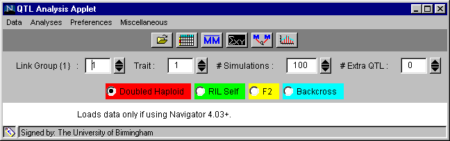
We will first give you an overview of the options available on the applet and then go into more detail as we work through the example. The applet window will always appear as shown in Figure 1.

Figure 1. The applet window set for example 1, Brassica DHLs, linkage group 1 and trait 1.

Beneath the title bar are five horizontal fields controlling different aspects of analysis.

Field 1: 4 clickable menus. The choices revealed by clicking on these are shown below.

Data	Analyses	Preferences	Miscellaneous
Load	Marker Means	Means as Symbols	Trait Distribution
Edit	Marker Regression	Kosambi Mapping Function	Map®
Sort Markers	Interval Mapping	File Format	Draw
	Expected	Calculate Trait	Add QTL
		Allow Dragging	Clear List
		Colours	About

Clicking on one of the choices in a menu will activate it and cause the menu to disappear. Three of the options in the Preferences menu (Means as Symbols, Kosambi Mapping Function and Allow Dragging) are 'checked' items - if you select one by clicking on it, it will be activated and the menu will disappear but if you look at the menu again this item will appear with a tick beside it showing that it is functioning. Clicking on the item again will de-select it and the tick will be removed.

Field 2: 6 buttons. These are shortcuts to some of the main options listed above. A description of their function will appear in Field 5, the white line at the bottom of the applet, when the cursor is held above them. Select a button by clicking on it with the mouse.

Open folder	= load data
Spreadsheet	= view and edit data
MM	= single marker ANOVA
S XY	= marker regression analysis
M-Q-M	= interval mapping analysis
Bar chart	= expected

Field 3: 4 boxes with scroll bars, whose values can be altered with the up/down arrows to their right or with the keyboard. (Press the return or enter key for the change of value to be recognised if you are using the keyboard method.)

Link group { }	choose the linkage group you wish to examine
Trait	choose the trait you wish to examine
Simulations	choose the number of simulations you wish to use to provide confidence intervals for the marker regression analysis
Extra QTL	choose the number of additional QTL above the default single QTL you wish to fit to the given linkage group (i.e. the value 0 here means that 1 QTL will be fitted.)

Field 4: 4 radio buttons, one for each of the four population types:

Doubled haploid RILSelf F2 Backcross

The default is doubled haploid, but you must remember to select the correct one for the population you are analysing. If you look at any of the other examples, you must specify the population type with these buttons before doing the analyses.

USING THE APPLET TO WORK THROUGH THE AN EXAMPLE

Example 1 involves 150 DHLs of Brassica oleracea, 2 quantitative traits and 84 markers across the 9 linkage groups. These data for the line means for each trait will be automatically loaded for you when you start. We will explain how to load your own data later.

Prior analysis

Before the data were loaded, an ANOVA was performed with a standard statistical package to establish that the lines differed significantly for these quantitative traits and to obtain a value for the additive genetical variance, V_A.

Viewing and editing data

The data for this example are already loaded and can be viewed in spreadsheet form using either the 'edit' facility or the spreadsheet button. You can move around the spreadsheets using the scroll bars.

The marker data are in the larger spreadsheet and the trait data are in the smaller one. Clicking on a spreadsheet will bring it to the front. A spreadsheet can be moved around the screen by clicking and dragging on the title bar. Each row has the data for a different line.

Marker sheet:

Row 1	Value. This box enables you to change genotype data - see below.
Row 2	Marker name. Although marker names of any length are acceptable, the whole name may not be visible due to the cell size.
Row 3	Position of marker in centimorgans (cM) on the linkage group (chromosome) shown on Row 3.
Row 4	Linkage group on which the marker is positioned
Row 5	Number of lines with missing genotype data for that marker. This helps in the decision of whether to exclude a marker from the analyses.
Row 6	Segregation ratio of the two alleles, given as nAA:nBB. This will indicate if there is segregation distortion for that marker. Where there are no BBs, e.g. Example 4, backcross data, the ratio will appear as nAA:0.
Row 7 etc	Genotype data. In this example, the data are in the form: AA = 1, BB = 3, Missing = 4. There are no heterozygotes (AB = 2) as the lines are doubled haploids. Other notations are acceptable (see loading data) and the data will appear in the notation that you entered.
Column 1	The line (or individual) number, which is assigned in the order in which the data are entered.

Trait sheet:

Row 1	Trait names, if these have been entered. The size of the cell will prevent viewing of the whole of a long name.
Row 2 etc.	Trait means. Missing values are in the form '-' but other notations are acceptable (see loading data).
Column 1	The line (or individual) number, which is assigned in the order in which the data is entered.
Column 2 etc.	Each trait appears in a different column, in the order in which they were loaded.

Markers and/or lines (individuals) can be selected for exclusion from the analyses. Use the scroll bars on the spreadsheet to bring the marker name or line number into view. Move the cursor to the marker name in Row 2 or the line number in the first column and double-click. The cell will turn red, signifying that this marker or line has been excluded. Double-clicking on a red cell will deselect it, returning it to normal colour and including the marker or line in subsequent analyses.

Reasons for selecting markers: Although the genetic map of B. oleracea that we used had 310 loci, the data for only 84 of the loci were entered.

Where possible, markers that were 10 to 15 cM apart were selected. For most QTL analyses, this spacing is quite sufficient and more markers do not help. It is best to use markers which are scored in most individuals and which are known to be most reliable. It may be necessary to exclude some of your markers before entering the data, particularly when the map has a large number of loci as it will not be possible to enter more markers for any one linkage group than there are number of lines.
The information on map distances, number of missing data points and segregation ratio displayed in the spreadsheet may help you to decide which others to exclude. Distorted segregation, away from the expected ratio (1:1 in a DH population), can arise from the differential survival of the two alleles or the misclassification of the genotypes.
Distortion due to selection will affect all linked loci in inverse relation to their distance from the affected locus whereas distortion due to misclassification will normally only affect the locus concerned. Therefore, if a marker shows a high level of segregation distortion which is not accompanied by similar levels of distortion in closely adjacent markers then this is likely to be an unreliable marker and should be excluded.
Although there is an option to exclude markers in the software, this will not affect your original data files, so if you plan to reload the data on another occasion and want to exclude the same markers, it would be wise to create a new set of data files.
Running the analyses with large numbers of markers will take more computing time and will not give a more reliable estimate of the position of a QTL. The precision of QTL location depends more on sample size than on the density of markers. Although the analyses will give a position for the QTL, the 95% confidence intervals associated with it can span 30cM or more.

Changing genotype values: Genotype scores can be changed within the spreadsheet.

Click on the cell that you wish to change and the value in that cell will appear in the 'value' box in Row 1.
Delete the score in the 'value' box, enter the new score and press the return or enter key. The new value will then appear in the genotype cell.
The effect of the changes can be assessed by rerunning the analyses.
You cannot return to your original scores unless you type them in again (pressing enter each time) or you reload your data files (which will not be altered). If you wish to make a permanent change in your genotype scores you must do it in your data file.

Displaying and saving results

Once an analysis has been selected, the results are displayed in a window, similar to the one shown in Fig 2, which is from the analysis of linkage group 2 with trait 1 by Marker Regression.

N.B. Do cancel a window when not needed as it takes up RAM. Since the windows can be hidden behind the browser window, it is a good idea to minimise the browser so that the Applet can be used like a toolbar and output can be seen at all times. In Windows 95 all current results windows are shown on the status bar.

Windows can be moved around the screen by clicking and holding the left hand mouse button on their blue title bar and dragging the window to the required position. This enables you to put windows side by side to compare their results.

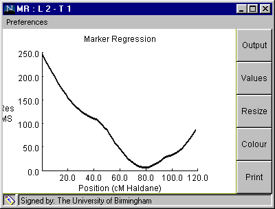
Fig 2. Typical analysis output window.

At the top right of the window are the usual minimise, maximise and cancel buttons. At the top left is a title, with an abbreviation of the analysis, the linkage group and the trait if applicable. On the right hand side are five buttons and under the title bar is a 'preferences' menu. These five buttons allow the following operations.

Output

toggles between graph and text output. Maximise the window and/or use the scroll bars to see the full content of the text output.

Values

tabulates x and y co-ordinates on the text output area

Resize

resizes the window to its original shape if it has been shrunk, stretched or maximised. Shrinking or stretching can be achieved by moving the mouse arrow to the edge of the window. When it changes to a double headed arrow, click and hold down the left hand mouse button and drag the window edge to the required position.

Colour

toggles between the default colours of the graph and black and white. Alternative colours can be selected using the 'colour' option in the 'preferences' menu on the Applet itself.

Print

sends the contents of the window directly to the printer. The size of the printout of the graph depends on the size of the window. The size of text output does not change with window size. The title bar and the buttons do not appear on the printout.

Axes

clicking on 'preferences' on the menu bar below the title bar of the window will reveal an 'axes' option which allows you to change the axes settings. Clicking on 'axes' will show a table giving the maximum, minimum and interval points on the x and y axes. Clicking in a cell will allow you access to alter its value but you must press the return or enter key for the change to be recognised. When you have made all your changes click in the 'apply' box, to produce a tick, and then cancel the axes window. The axes will change to your settings once the axes window has been cancelled.

A Java security window may appear when you try to view the text output or if you print directly from a window. It will warn that the applet is requesting permission for the high risk activity of reading and writing to the system clipboard for your computer or for the low risk activity of printing. Click on 'grant'.

The text output is written directly to your clipboard. You can paste the contents of the clipboard straight into another application such as a word processing package. A result window containing a graph can be copied to the clipboard by pressing Alt and Print Screen on the keyboard simultaneously and it can then be pasted into a document, but in this case the whole window complete with title bar and buttons will be copied. If several windows are open, only the currently selected one, with the blue title bar, will be copied. It is useful to have a 'Word' document open, or minimised on the status bar, to receive each result that you wish to save. When the text is pasted it may not appear as on screen and you may need to insert or remove tab spaces or change the font size to align the headings and figures correctly.

The display in the 'marker means' and 'expected' results windows can be changed from vertical bars to square symbols by selecting Means as Symbols in the Preferences menu, if desired. If selected, this item will appear with a tick, when the menu is next viewed.

Prior to analysis

Population type: Once the data have been loaded but prior to any analysis, the population type must be defined by clicking on one of the buttons in Field 4 of the applet. For this example, it is the default, doubled haploid option.

Mapping function: If the Kosambi rather than the Haldane mapping function has been used to calculate the map distances between the markers, the Kosambi option must be selected by clicking on Kosambi in the Preferences menu. A tick will appear beside it to show that it has been activated. This is necessary for the Marker Regression analysis as the map distances are used to calculate the recombination frequencies. Graph axes will be labelled cM Haldane or cM Kosambi depending on whether the default or Kosambi has been chosen. The maps for all the examples are based on the Haldane mapping function.

Select the linkage group and the trait you wish to examine.

Trait Distribution: You can check whether the selected trait has a 'normal distribution' by selecting trait distribution in the Miscellaneous menu. A distribution graph will appear in a result window. The values button on the window will tabulate the x and y coordinates and the output button toggles between the graph and statistics about the distribution, such as the mean, variance, skewness and kurtosis. The data for both traits in Example 1 follow a normal distribution. If your own trait data do not show a normal distribution you can use the 'calculate trait' option to adjust or transform the data.

Trait manipulation: The calculate trait item in the Preferences menu allows you to produce a composite trait using existing trait values, for example combining leaf length and leaf width to give leaf area. It also allows you to produce a transformed trait from an existing trait. Frequency distributions skewed to the right are often made more symmetrical by transformation to a logarithmic scale. The square root of the values for a trait such as surface area may have a more normal distribution than the area values themselves.

Operators are: + - / * ^ (to the power of, i.e. 2^3 = 8), functions are LN (natural logarithm) LOG (base 10 logarithm) SQRT (square root) EXP (exponential) and constants are PI (3.1415927) and E (2.7182818). Round brackets can be used to group calculations. The precedence of operators is that normally found in computing languages so that multiplication/division has a higher precedence over adding and subtracting e.g. 1+2*3 = 7 and (1+2)*3 = 9

When in doubt, use brackets. The letter T followed by a number n indicates that the value of the nth trait should be substituted in the calculation, thus T2*PI will multiply trait two by PI (3.1415927). The enter key must be pressed for the entry to be registered and the 'Apply' box must be checked for the equation to be used in subsequent analyses. You must uncheck the Apply box before you can work with the next trait.

An example of how to enter a complex expression into the trait calculator is:

PI*SQRT(EXP(LN(T1))^2) press enter, click apply then OK. T1 indicates trait 1, squaring cancels the square root and the exponential function cancels the natural logarithm so the result is trait 1 multiplied by PI. Obviously, T1*PI will achieve the same outcome but this illustrates how you can build up an expression.

QTL Analysis

You are now in a position to analyse the data for the trait and linkage group you have selected. For this example we have selected, linkage group (i.e. chromosome) 2 with trait 1 because this linkage group has a QTL for trait 1.

Single marker ANOVA

Using the 'marker means' option in the Analyses menu or the MM button, a preliminary analysis can be carried out. This looks at all individual associations between markers and phenotype.

Theory: For each marker, the mean of the trait scores for all those lines homozygous for the allele from parent 1 is compared to the mean trait score for all those lines homozygous for the allele from parent 2 and to the mean of those heterozygous for this marker.

If a marker is on a different chromosome to any loci affecting this trait, QTL, the alleles for the QTL will segregate independently of the alleles for the marker. Because the collection of lines homozygous for the marker allele from parent 1 will have all possible QTL allele combinations, the mean trait score will be similar to the population mean. This also applies to the other two marker genotype classes so the mean trait scores of the three classes will not differ significantly from one another.
If a marker is close to a QTL, then most of the lines homozygous for the marker allele from parent 1will also be homozygous for the trait allele from parent 2. Similarly, most of the lines homozygous for the marker allele from parent 2 will also be homozygous for the trait allele from parent 2.
Therefore, the mean trait scores for these two classes will differ and an ANOVA can be used to test whether the difference is significant.
The size of the difference will depend on the effect of that QTL, a, and how close the marker is to the QTL. The difference between the genotypes will be maximal and equal to 2a if the marker and the QTL co-segregate.
Because only one marker at a time is examined for its association with the trait, the single marker analysis has some limitations:

the magnitude of the QTL effect is underestimated because of recombination between the QTL and the marker; tight linkage of a marker to a QTL with small effect cannot be easily distinguished from loose linkage of a marker to a QTL with large effect;
although the chance of a false positive at any given marker locus is only 5%, the chance that at least one false positive will occur over the entire genome is much higher; and when more than one QTL are present on a chromosome the power of the ANOVA will be decreased.

However, it is a useful first step.

Results of analysis

When the analysis has been selected, a result window will appear (Fig 3), with a graph showing the additive effect associated with each of the nine markers in linkage group 2.

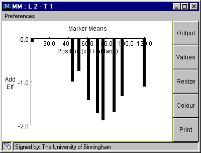
Fig. 3. Window with graphical output from "Marker Means" analysis

Interpretation of Window in Fig 3.:

The position of each marker on the linkage group is shown in centimorgans (cM) on the x axis.
The graph shows that the additive effect is greatest close to marker 6 at around 75 cM, suggesting that if there is a QTL present, it is close to marker 6.
Clicking on the output button presents the data on which the graph is based (Table 1). It shows the marker positions, the additive effect associated with each marker, the mean trait score for each marker genotype, i.e. M1M1 mean and M2M2 mean (there are no heterozygotes, M1M2, as the data is from DHLs), and the number of lines of each genotype.
It also gives the results of a one way ANOVA, testing for differences between the 2 marker means for the trait. There are highly significant additive trait effects associated with markers 5 and 6 and a less significant one with marker 7. (The additive effect is half the difference between the trait means of the two homozygous marker genotype classes and it will be negative if parent 1 has the allele which is associated with a lower trait score)

Table 1. Data displayed on clicking "Output" button shown in Fig. 3.

Marker Positions and Trait Means:

Linkage Group: 2 Trait: 1 No. Pos. Add. eff. mean(11) n(11) mean(12) n(12) mean(22) n(22) F P 1 0.0 -0.08 32.29 74 0.0 0 32.45 54 0.018 0.8925 NS 2 42.4 -1.0 31.45 66 0.0 0 33.46 77 3.344 0.0696 NS 3 49.5 -0.76 31.67 65 0.0 0 33.19 83 1.843 0.1767 NS 4 59.5 -1.43 30.65 53 0.0 0 33.51 79 6.286 0.0134 * 5 68.8 -1.73 30.21 49 0.0 0 33.67 99 9.051 0.0031 ** 6 74.8 -1.9 30.09 52 0.0 0 33.9 95 11.303 0.0010 *** 7 86.5 -1.71 30.05 48 0.0 0 33.47 97 9.102 0.0030 ** 8 95.1 -1.34 30.66 42 0.0 0 33.33 104 4.72 0.0315 * 9 118.4 -1.12 31.17 50 0.0 0 33.41 91 3.52 0.0627 NS

Table 2 illustrates the corresponding form of the data for an F2 example in which heterozygote and dominance effects are dispalyed.

Table 2. As for Table 1 but for an F2 population.

Marker Positions and Trait Means Linkage Group: 1 Trait: 1 No. Pos. Add. eff. Dom. eff. mean(11) n(11) mean(12) n(12) mean(22) n(22) F P 1 0.0 0.6 -1.19 43.23 31 41.44 51 42.03 18 2.442 0.0923 NS 2 11.0 0.73 -1.2 43.4 28 41.46 52 41.93 20 2.75 0.0689 NS 3 22.0 1.55 -1.06 43.94 32 41.33 54 40.84 14 7.007 0.0014 ** 4 33.0 2.7 0.02 44.33 36 41.65 45 38.94 19 20.182 0.0 *** 5 44.0 3.86 0.8 44.8 36 41.75 48 37.08 16 52.919 0.0 *** 6 55.0 5.31 1.45 45.46 34 41.6 54 34.84 12 193.281 0.0 *** 7 66.0 3.65 0.27 45.13 29 41.75 55 37.82 16 38.048 0.0 *** 8 77.0 2.98 0.52 44.49 31 42.04 49 38.54 20 24.416 0.0 *** 9 88.0 3.21 0.84 44.66 26 42.3 54 38.24 20 27.84 0.0 *** 10 99.0 2.39 0.68 44.12 25 42.41 51 39.33 24 14.137 0.0 ***

Marker Regression

This follows the method proposed by Kearsey and Hyne (1994) and tries to locate the QTL with respect to all markers simultaneously by regression onto the marker means. It also estimates the additive (and dominance) effects, tests their significance and tests for more than 1 QTL.

Significance tests and confidence intervals are obtained by simulation, and the user can vary the number of simulations.

For a quick initial scan, 100 simulations (the default) may be enough to indicate whether there is a QTL on the chromosome.

If there is, additional simulations, e.g. 1000, may be needed to accurately determine probability levels and confidence intervals.

N.B. The probability values associated with F tests are not the same as those taken from statistical tables because of correlations between the Marker Means.

Clicking the (S XY) button will produce the window shown in Fig. 4

Fig. 4. The Marker Regression window

The Marker Regression Window displays the values of the Residual MS from the Regression ANOVA for all possible QTL positions. In the data displayed in Fig 4, the Residual MS reaches a minimum at 80 cM. This would be the most likely position for the QTL if there is one.

Clicking on the "OUTPUT" button gives the data and anlyses shown in Table 3. They are based on 100 simulations.

The Corresponding output with 1000 simulations is shown in Table 4 for comparison.

Table 3. Marker regression analysis from clicking on "OUTPUT" button on Fig. 4 (100 simulations).

Linkage Group: 2 Trait: 1 QTL located at 80.0 cM Additive effect = -1.9991219 Source df MS F P Add Reg 1 2355.68 75.22 0.0 Residual 7 6.62 0.21 0.838 Error 139 31.32 Simulated QTL position is 78.747 +/- 11.167 Simulated Additive QTL effect is -2.007 +/- 0.666

etc

Table 4. Marker regression analysis from clicking on "OUTPUT" button on Fig. 4 (1000 simulations).

QTL Mapping by Marker Regression: Result Linkage Group: 2 Trait: 1 QTL located at 80.0 cM Additive effect = -1.9991219 Source df MS F P Add Reg 1 2355.68 75.22 0.0050 Residual 7 6.62 0.21 0.834 Error 139 31.32 Simulated QTL position is 77.98 +/- 15.292 Simulated Additive QTL effect is -2.052 +/- 0.609

The analyses in tables 3 and 4 show the following:

There is a significant regression (P=0.005) indicating a single QTL

The Residual MS is not significant (P=0.834) indicating that there is no evidence for additional QTL.

The most likely location for the QTL is at 80.0cM with an additive effect of 1.999 units (days to flowering in this case)

The fact that the additive effect is negative indicates that P2 has the increasing allele.

Twice the standard deviation of the QTL location is estimated to be 15.92 units giving a 95% confidence interval of approximately 32 cM; i.e. between 64 to 96 cM.

The P values automatically take into count the number of tests performed on that chromosome, but allowance need to be made for the fact that one is looking at several chromosomes and several tests. It is therefore good practice to use at least P<0.01 for significance to avoid Type 1 errors.

To plot this QTL on a map.

Click on Miscellaneous menu and bring up Map and Draw map.

Repeat but choose "Add QTL".

Repeat Draw map.

This produces the map as in Fig 5.

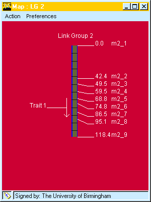
Fig. 5. QTL drawn to map. The direction of the arrow indicates it P1 has the decreasing allele, the horizontal line indicates the QTL location and the length of the arrow gives the confidence interval. Marker names and positions are also indicated.are .

Interval Mapping

This can be addressed by clicking the MQM button and results in the window shown in Fig 6.

The analysis follows the method described by Haley and Knott (1992).

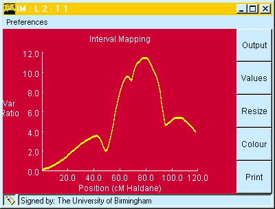
Fig. 6. Output from "Interval Mapping" showing Variance Ratio for the regression plotted against map. position.

Table 5. Output from clicking "OUTPUT" button on window shown in Fig 6.

QTL Mapping by Interval Mapping: Result 1 QTL

Linkage Group: 2

Trait: 1

QTL located at 79 cM

Test Statistics : F 11.493 LR 11.2146

Res. SS - Full Model 6262.181 d.f. 146

Res. SS - Red. Model 6755.136 d.f. 147

Mean 31.8945

Add Eff. -2.0071

Taken together ( Fig. 6 and Table 5) we find:

The most likely location for the QTL is at 79cM

The F test statistic for regresssion is 11.493 for 1 and 146 df (P<0.001)

The estimated effect of the QTL is 2.007 units (days)

P1 has the decreasing allele because a is negative.

These values can be compared with those given above for Marker Regression in Table 2.

QTL can be added to the map as before.

Comparison of observed and expected marker means.

When either the Marker Regression or Interval Mapping analyses have been run, the observed marker means can be compared to their expected values (based on the mapped QTL and their additive effects) by use of the "Bar chart" button on the applet or by choosing "expected" from the analysis menu, as shown in Fig. 7.

The "Expected" graph will always be produced using the QTL locations and effects estimated in the last analysis attempted.

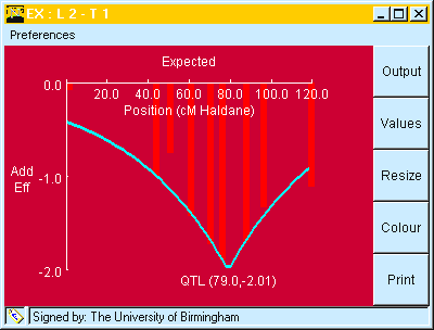
Fig. 7. Window showing observed marker means (Vertical bars) at different chromosome positions compared to their expected values (blue line). The expected values were taken (automatically) from the interval mapping analysis, shown in Table 5.

Candidate loci comparisons: If the "Allow dragging" item in the "preferences menu is checked, then it is possible to move the expected line by "click and drag" with the mouse to the position of the possible candidate locus. This allows you to see how well it fits the candidate.

Loading data

Once the Applet has appeared, after selecting any of the four example sets, your own data can be loaded.

Data files

Three data files are required; all with the same file name but with different extensions. At present, Unix users are advised to use lowercase letters for their directory and file names when using this software.

filename.gen -

genotype data

filename.mrk -

marker data

filename.tra -

trait data

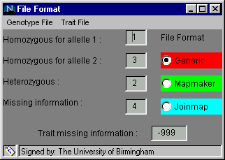
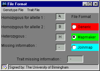
The software is designed to accept several different formats in order to minimise the number of alterations you will need to make to your data. The File Format dialog box, found in the Preferences menu and shown below, is used to inform the software of the format of your data, before you try to load it.

Options available under the headings on grey menu bar:

Genotype file

Trait file

- individuals as cols

- traits as rows

- marker names

- trait names

One of three formats, generic, Mapmaker or Joinmap, can be chosen by clicking on the radio button beside the name (the default option is generic). When one is selected, the default genotype coding and missing trait coding are inserted into the text boxes but these can be altered if your data has different codes. The default codings for the generic format and the Mapmaker format are shown above. To alter a code: click on the relevant cell, delete the entry, insert your own code, press enter or return for the change to be registered and move on to the next cell.

Genotype file

A generic genotype file is shown on the left below. The first row always contains three numbers, representing the number of individuals (n-ind), the number of markers (n_mrk) and the number of traits (n_tra). Then follows n_ind rows of individuals (lines), each row containing the genotype at each marker locus of the individual. The genotypes are coded: 1, homozygous for parent 1; 2, heterozygous; 3, homozygous for parent 2 and 4, missing data. The data can be delimited by tab characters, spaces or commas. Other codes will be accepted if you change the default code in the File Format box as explained above.

If your data has the individuals as columns (= markers as rows), click on 'individuals as cols' in the 'genotype file' menu in the File Format box, before loading the data.

If you have included marker names (at the top of each column in the default orientation or at the start of each row in the 'individuals as columns' option), click on 'marker names' in the 'genotype file' menu of the File Format box.

If you have not included marker names make sure the order of the markers is the same in the genotype file and the marker file. If marker names are included but the order is not the same in the two files, a message informing you that there are marker name mismatches will appear when you load the data. It will suggest that you use the menu option to sort the data. Clicking on OK at the end of the message does not sort the data, you must go to the 'data' menu on the Applet menu bar and select sort. The data will be loaded whether or not you select this option. Only use the sort option if you are sure the markers are in a different order in the two files. If you get the message when you think the order should be the same, check your data files carefully. The marker order in the marker file will be taken as correct and the .gen data sorted accordingly.

An example of a genotype file in Mapmaker format is shown below. An extra heading line giving the data type is included but you must define the population type in the Applet as well. Marker names are expected, prefaced with an * , and the genotype data for any individual are in a column. The options 'individuals as cols' and 'marker names' do not have to be selected.

A genotype file in Joinmap, Mapmaker and generic formats are shown below:

JOINMAP FORMAT

name = Arab popt = SSD nloc = 67 nind = 98 ntra = 3 # more comments # and again # next line 2 spaces #next line 2 tabs g4715-a abbaababbb abaab-abbb aa-bbbaaab baabbaabaa babbaabb-a babbbbbaaa baaaaababa bbbbaaaaaa bba-abaaaa bbabbbbb m488 abbaababbb abaab-abbb aaabbbaaab baabbaabaa babbaabb-a babbbbbaaa baaaaababa bbbbaaaaaa bbaaabaaaa bbabbbbb g3786 aaaaababab ababbaabbb aaabbbaaab baabbaa-aa babbaabb-a babbbaaaa& baaabababb bbabaaabba -ba-bbaaa- bbabbbbb g3829 aaaaababab ababbbabab aa-bb-aabb bbabbaaaab babbabab-a aaaabbaaaa baaa--babb bbbbaaabba -ba-bbb--a bbab--ab

etc.

MAPMAKER FORMAT

data type ri self 98 67 3 # more comments # and again # next line 2 spaces #next line 2 tabs *g4715-a abbaababbb abaab-abbb aa-bbbaaab baabbaabaa babbaabb-a babbbbbaaa baaaaababa bbbbaaaaaa bba-abaaaa bbabbbbb *m488 abbaababbb abaab-abbb aaabbbaaab baabbaabaa babbaabb-a babbbbbaaa baaaaababa bbbbaaaaaa bbaaabaaaa bbabbbbb *g3786 aaaaababab ababbaabbb aaabbbaaab baabbaa-aa babbaabb-a babbbaaaa baaabababb bbabaaabba -ba-bbaaa- bbabbbbb *g3829 aaaaababab ababbbabab aa-bb-aabb bbabbaaaab babbabab-a aaaabbaaaa

etc

GENERIC FORMAT

25 3 1 1, 3, 3 1, 3, 3 1, 1, 1 3, 3, 3 3, 3, 3 1, 3, 1 1, 1, 3 1, 1, 1 3, 3, 3 3, 3, 3 3, 3, 1 1, 1, 1 3, 3, 1 3, 3, 3 1, 1, 1 3, 1, 1 3, 3, 3 3, 3, 3 1, 1, 3 1, 1, 3 3, 3, 3 3, 3, 3 3, 3, 1 1, 1, 3 3, 3, 3

Marker File

The marker file contains all the markers you have chosen for all the linkage groups. Markers spaced approximately 10 to 15 cM apart are sufficient. Please read the section on page 4 concerning the choice of markers. Marker names can be any length but do not use spaces or commas within a name. If you are using data in Mapmaker format, do not include the asterisk (*) at the start of the marker name in the marker file.

Column 1 contains the marker names.

Column 2 contains the marker linkage groups denoted by an integer number starting at 1.

Column 3 contains the respective marker positions.

The data can be delimited by tab characters, spaces or commas.

A typical marker file is shown below for markers on 5 linkage groups.

g4715-a, 1, 0.0 m488, 1, 0.0 g3786, 1, 8.0 g3829, 1, 16.5 m235, 1, 20.1 m253, 1, 33.4 gapB, 1, 48.8 m213, 1, 63.2 g4026, 1, 72.5 m315, 1, 82.1 g4552, 1, 88.5 m532, 1, 103.4 g17311, 1, 109.2 m246, 2, 0.0 g4553, 2, 2.1 g4532, 2, 6.0 g4133, 2, 9.9 m216, 2, 16.0 m251, 2, 22.6 g6842, 2, 29.5 er, 2, 32.2 m220, 2, 38.0 m323, 2, 43.6 g17288, 2, 43.6 g4514, 2, 49.1 m336, 2, 52.9 m583, 3, 0.0 g4523, 3, 0.6 m228, 3, 7.6 g4708, 3, 7.6 m105, 3, 11.6 g4711, 3, 20.7 m249, 3, 37.8 g4117, 3, 37.8 g4564-b, 3, 41.2 g4014, 3, 43.9 m457, 3, 48.1 g2778, 3, 53.3 m424, 3, 57.3 g3843, 4, 0.0 g2616, 4, 4.9 m506, 4, 4.9 m518, 4, 14.9 pCITd23, 4, 18.1 g6837, 4, 26.6 g10086, 4, 27.7 g4564-a, 4, 27.7 m326, 4, 28.7 m226, 4, 32.0 g3845, 4, 32.5 m600, 4, 43.8 g8300, 4, 48.4 g3088, 4, 50.3 pCITd99, 4, 53.3 g3713, 4, 64.6 g3715, 5, 0.0 m217, 5, 4.5 g3837, 5, 5.5 CHS, 5, 10.7 g4560, 5, 17.1 m291, 5, 20.3 g4715-b, 5, 27.6 m247, 5, 58.1 g4028, 5, 62.5 m435, 5, 81.2 g2368, 5, 88.8 m555, 5, 94.7

Trait file.

The software expects a trait file with the following format: each column represents a single trait and contains the trait values for all the individuals; names of the individuals and trait names are not included.

If you include the trait name at the top of each column, click on 'trait names' in the 'trait file' menu in the File Format box before loading the data.

If you have the traits in rows rather than columns (with the trait name at the start of the row, if included), click on 'traits as rows' in the 'trait file' menu in the File Format box (and 'trait names', if included).

If you are using a code for missing trait values that is different to the default one in the option you are choosing in the File Format box, remember to alter the code in the box before loading the data. (Never use zero as a code for missing trait values).

The individuals in the trait file should be in the same order as in the genotype file.

The data can be delimited by tab characters, spaces or commas. A typical trait file for 3 traits (columns) is shown below:

248.1 238.75 263.6 348.4 357.2 268.6 371.7 353.2 336.7 317.7 351.75 282.4 367.7 370.3 336.2 430.7 423.7 362.7 276.7 281.2 240 211.1 240.5 194.33 449.3 445.8 345.6 248.8 226.3 247 407.7 441.3 351.8 230.2 171.7 184.2 195.9 171.3 187.2 362.3 390.8 318.3

etc

Check list

Check your three data files have the same file name with the correct file extensions.

Select the format which corresponds to your data, in 'file format' under 'preferences'. Make any alterations in the boxes if the data are coded differently. Use the options on the grey menu bar [individuals as columns, marker names, trait names or traits as rows] if necessary.

Click on the button showing an open file or 'data' and then 'load'.

If a Java security window appears, select 'grant'

A load window requesting direction to the data files may appear directly. If it is hidden, look on the status bar where active applications are displayed and a new label 'open' should have appeared; clicking on this will show the window. Open the folder in which your data files are stored.

Load the files by opening the .gen file or clicking on the group filename if this is displayed.

Use the sort option under 'data' on the menu bar, if prompted and it is appropriate.

Select the correct population type (default is dh).

Select kosambi if your map was produced using the Kosambi mapping function

Select linkage group and trait

View trait distribution

Use 'calculate trait' if necessary

Select marker means analysis

marker regression analysis

select number of simulations when doing marker regression

select extra QTL only if the results suggest that one QTL is not adequate

expected can use dragging if you require

map with QTL

interval analysis

extra QTL?

expected

map with QTL

Error messages found when loading data:

Error: trait exception: Unconvertible string 'Mean-1' has occurred at line 1 of the trait file

The trait headings (the first of which was Mean-1) had been left in the trait file. Either remove the headings or go to Preferences then File format then trait file and click on trait names. Then reload the data.

Error: trait exception: Unconvertible string '-' has occurred at line 8 of the trait file

The missing data in this trait file should have been entered as '-999' as these files were in the generic format but one on line eight was entered as '-'. This data point could be corrected but if all the missing data were entered as '-', they could either be replaced with ' -999' or the missing trait value in the box in the generic file format could be changed from '-999' to '-' (via Preferences, then File format)

Error: trait exception: null occurred when the 'tab' between two trait entries in a trait file was deleted, effectively causing the loss of a data point.

Error: An error has occurred in the genotype file header line

This message occurred when loading data in Mapmaker format without having changed the File format found in Preferences to Mapmaker.

It also occurred when entering data in generic form without the header line in the genotype file which specifies how many individuals, markers and traits there are.

Error: Unexpected character '1064' has occurred at line 2 of the genotype file

The name of the individual 1064 had been left at the start of line 2 in the genotype file (generic format). Names of individuals should be deleted.

Error: Unexpected character '11' has occurred at line 4 of the genotype file

One of the data points in line 4 of a generic genotype file had been entered wrongly as 11 instead of 1. Any unexpected character in the genotype file will be notified in this way with the line number specified (the header line is included in the count). Similarly an entry of 'c' instead of 'a' in a Mapmaker format genotype file will generate a similar message.

Error: Unexpected character m1-1 has occurred at line 2 of the genotype file

It is possible to include marker names in a generic format genotype file if Marker names is selected via Preferences, File format, Genotype file. An error message with the first marker name identified will occur if this selection is not done.

If a mistake is made in the genotype header line such that the numbers of individuals, markers or traits specified do not correspond with the numbers of individuals, markers or traits in the data, error or information messages will be generated. For example:

When entering the Arabidopsis data, which has 98 individuals, 67 markers and 9 traits, in Mapmaker format the following messages were displayed:

Information: 67 marker name mismatches, use menu option to sort; obtained when the number of individuals was entered wrongly as 100 (but the sort option should not be used in this case).

Error: Trait exception: null; obtained when the number of individuals was wrongly entered as 97.

Error; but with no explanation, was obtained when the number of markers was wrongly entered as either 65 or 69.

Error: Trait exception: null; obtained when the number of traits was wrongly entered as 8 or 10.

When entering the Brassica data in generic format without marker names in the genotype file or trait names the following messages were obtained when errors were made in the genotype header line:

Error; but with no explanation, was obtained when the number of individuals was wrongly entered as 149 instead of 150 and also when the number of markers was entered as either 82 or 86 instead of 84.

Error: Trait exception: null; obtained when the number of traits was entered wrongly.

N.B. When the number of individuals was entered as 180 instead of 150, the data was accepted. When the data was viewed via the spreadsheet button on the applet, the data for these non-existent individuals were displayed as stars in the genotype boxes and 0.0 in the trait boxes.

The following mistakes created in a Mapmaker format genotype file resulted in:

Information: 66 marker name mismatches, use menu option to sort. (The number relates to the number of markers affected although only one or two may be wrong)

No space between a marker name and its data.

One data point omitted.

A 'missing data' point entered as a space instead of a '-' (or other defined character).

An asterisk, *, was included at the start of each marker name in the marker file. Asterisks are expected in the genotype file of this format but not in the marker file.

Error: [but no explanation] occurred when a data point was omitted from a generic genotype file.

Information: 1 marker name mismatches, use menu option to sort.

Because both the genotype and marker files in the Mapmaker format contain the marker names, a mistake in a marker name in either will be identified. If the markers with their data have been entered in a different order in the two files the sort option can be used but if the error is a typing error of the marker name just correct the mistake. When marker names are included in a generic genotype file similar error messages will be obtained if the marker names in the genotype and marker files do not agree.

Error: Unconvertible string '8.0' has occurred at line 3 of the marker file was obtained when a linkage group was omitted from the third entry in a Mapmaker or generic format marker file . A similar message is obtained if a marker position is omitted.

The most common error is a missing data point in the genotype file. Please check your files carefully.

Output	toggles between graph and text output. Maximise the window and/or use the scroll bars to see the full content of the text output.
Values	tabulates x and y co-ordinates on the text output area
Resize	resizes the window to its original shape if it has been shrunk, stretched or maximised. Shrinking or stretching can be achieved by moving the mouse arrow to the edge of the window. When it changes to a double headed arrow, click and hold down the left hand mouse button and drag the window edge to the required position.
Colour	toggles between the default colours of the graph and black and white. Alternative colours can be selected using the 'colour' option in the 'preferences' menu on the Applet itself.
Print	sends the contents of the window directly to the printer. The size of the printout of the graph depends on the size of the window. The size of text output does not change with window size. The title bar and the buttons do not appear on the printout.
Axes	clicking on 'preferences' on the menu bar below the title bar of the window will reveal an 'axes' option which allows you to change the axes settings. Clicking on 'axes' will show a table giving the maximum, minimum and interval points on the x and y axes. Clicking in a cell will allow you access to alter its value but you must press the return or enter key for the change to be recognised. When you have made all your changes click in the 'apply' box, to produce a tick, and then cancel the axes window. The axes will change to your settings once the axes window has been cancelled.

filename.gen -	genotype data
filename.mrk -	marker data
filename.tra -	trait data

Genotype file	Trait file
- individuals as cols	- traits as rows
- marker names	- trait names